Why
Student: I finished the analysis and look at the great results! What do you think?
Ranae Dietzel and Andee Kaplan
Student: I finished the analysis and look at the great results! What do you think?
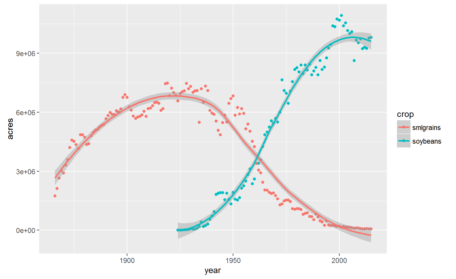
ggplot(both, aes(x=year, y=acres, group=crop, color=crop, shape=crop))+
  geom_point(size=3)+
  geom_smooth()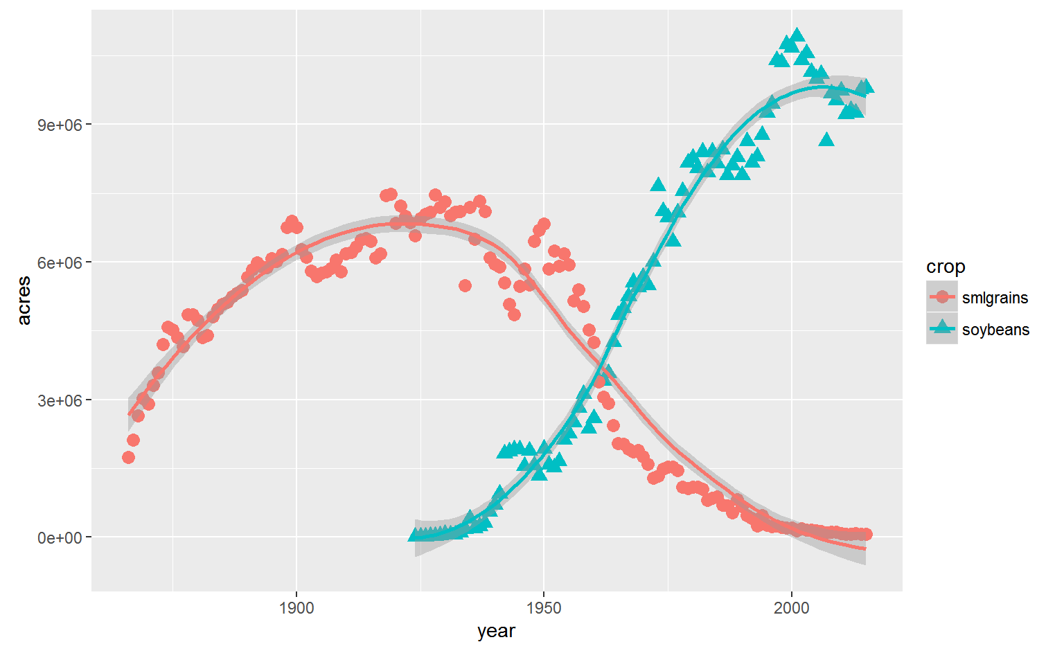
ggplot(both, aes(x=year, y=acres, group=crop, color=crop, shape=crop))+
  geom_point(size=3, alpha = .6)+
  geom_smooth()+
  ggtitle("Acres of small grains and soybeans in Iowa")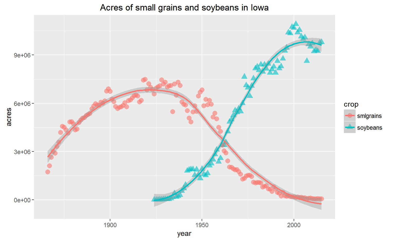
theme_set(theme_bw())
ggplot(both, aes(x=year, y=acres, group=crop, color=crop, shape=crop))+
  geom_point(size=3, alpha = .6)+
  geom_smooth()+
  ggtitle("Acres of small grains and soybeans in Iowa")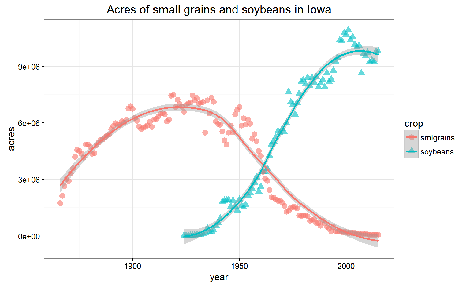
library(scales)##
## Attaching package: 'scales'## The following objects are masked from 'package:readr':
##
## col_factor, col_numerictheme_set(theme_bw())
ggplot(both, aes(x=year, y=acres, group=crop, color=crop, shape=crop))+
geom_point(size=3, alpha = .6)+
geom_smooth()+
ggtitle("Acres of small grains and soybeans in Iowa")+
scale_y_continuous(labels = comma)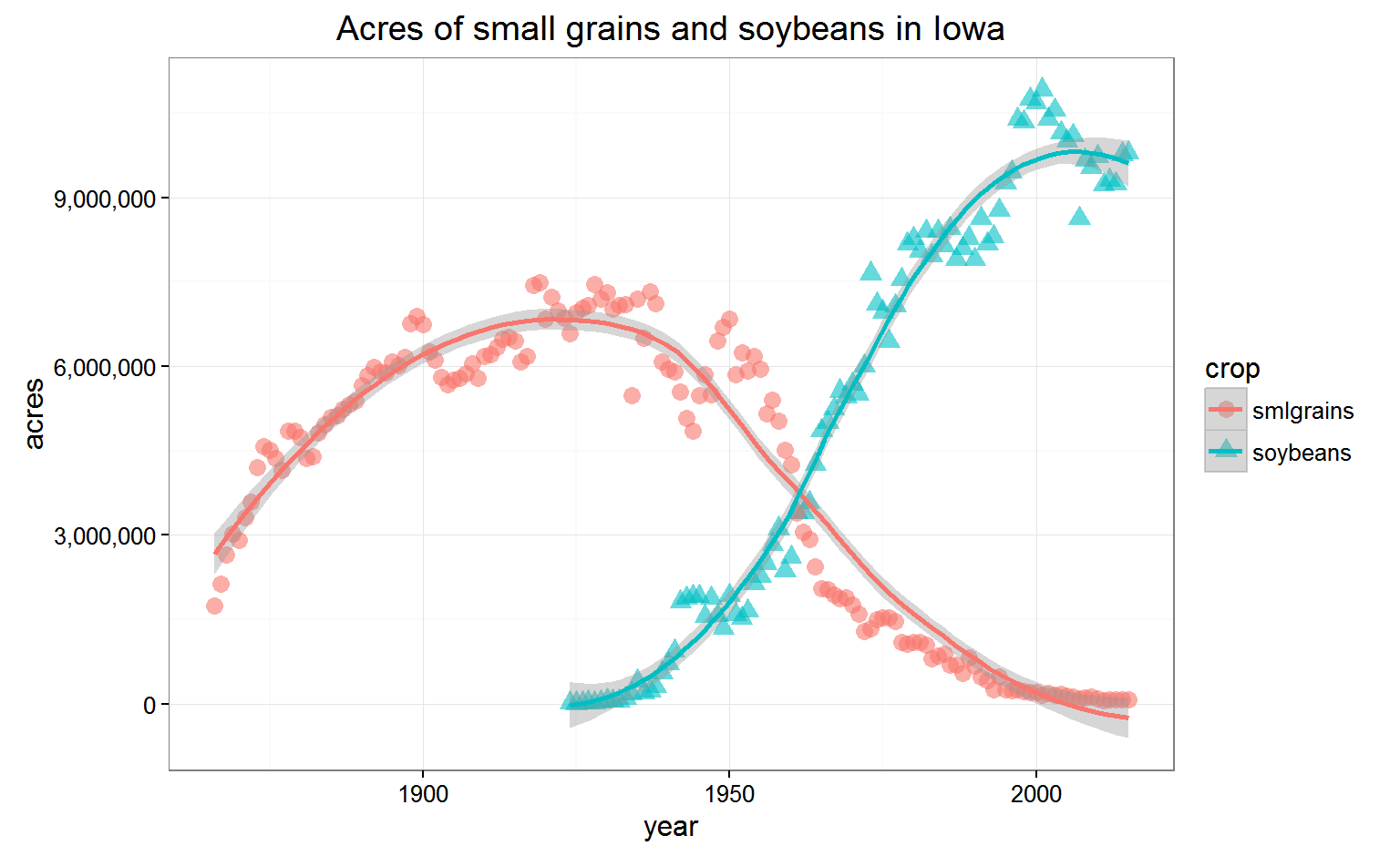
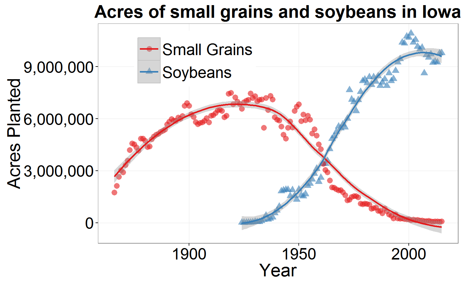
theme_set(my_theme)
ggplot(both, aes(x=year, y=acres, group=crop, color=crop, shape=crop))+
  geom_point(size=3, alpha = .6)+
  geom_smooth()+
  ggtitle("Acres of small grains and soybeans in Iowa")+
  scale_y_continuous(labels = comma)+
labs(x = "Year",y = "Acres Planted")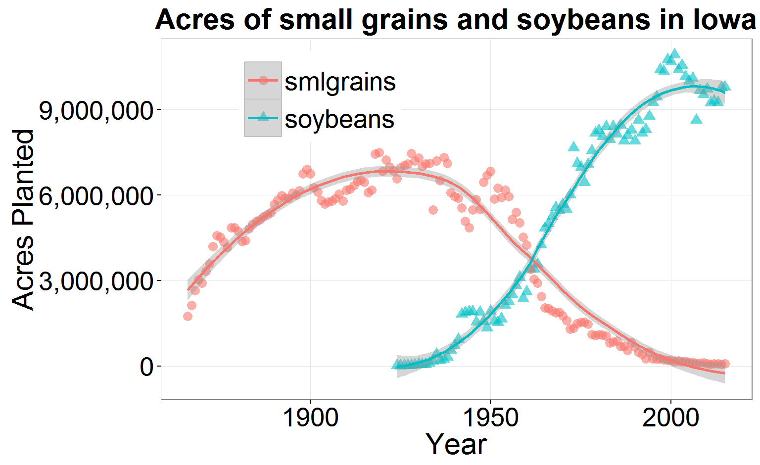
theme_set(my_theme)
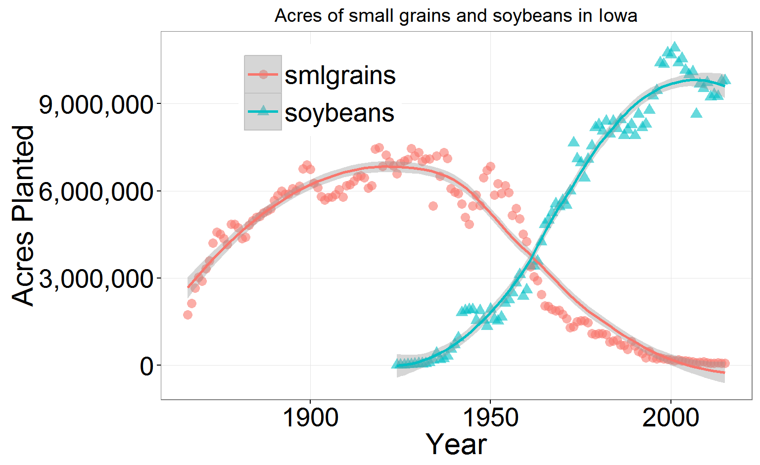
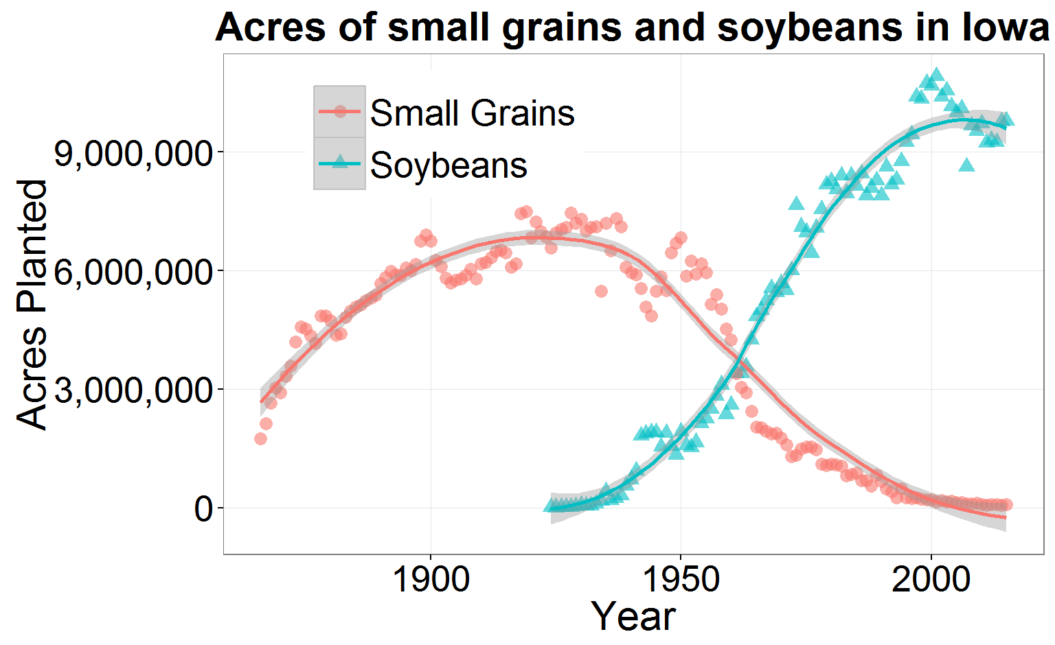
ggplot(both, aes(x=year, y=acres, group=crop, color=crop, shape=crop))+
geom_point(size=3, alpha = .6)+
geom_smooth()+
ggtitle("Acres of small grains and soybeans in Iowa")+
scale_y_continuous(labels = comma)+
labs(x = "Year",y = "Acres Planted")+
scale_color_discrete(name="Crop",
breaks=c("smlgrains", "soybeans"),
labels=c("Small Grains", "Soybeans"))+
scale_shape_discrete(name="Crop",
breaks=c("smlgrains", "soybeans"),
labels=c("Small Grains", "Soybeans"))

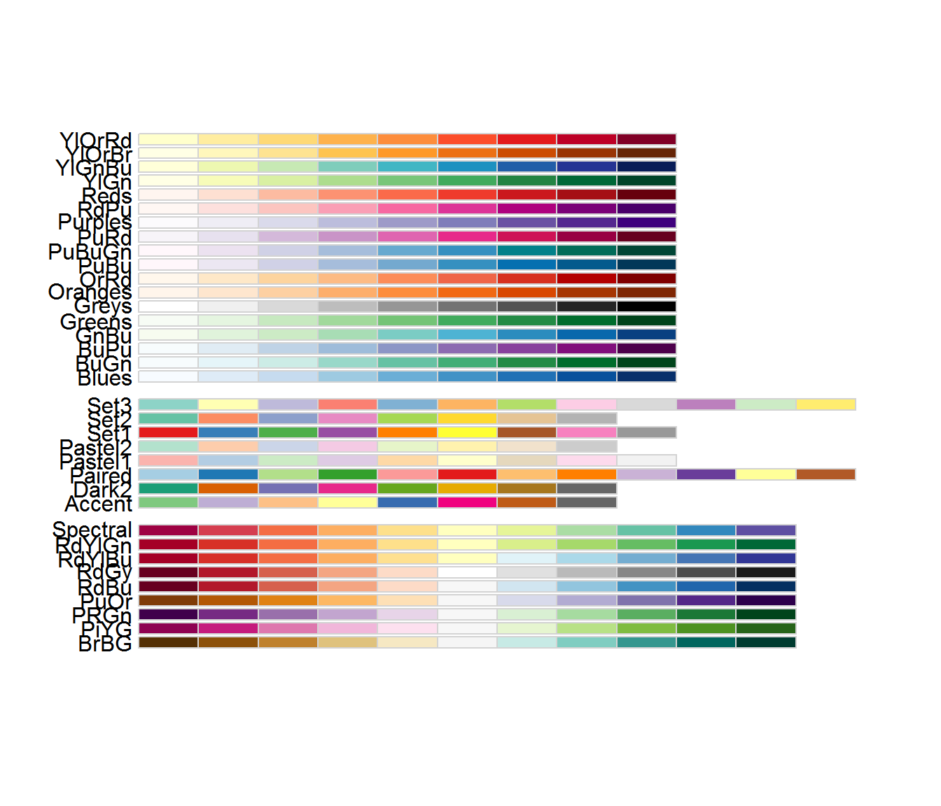
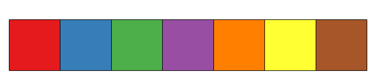
Qualitative schemes: no more than 7 colors
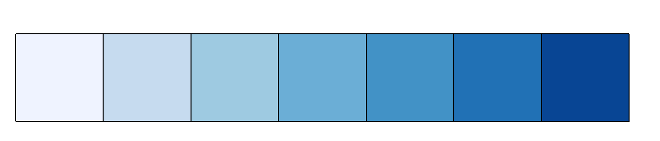
Quantitative schemes: use color gradient with only one hue for positive values
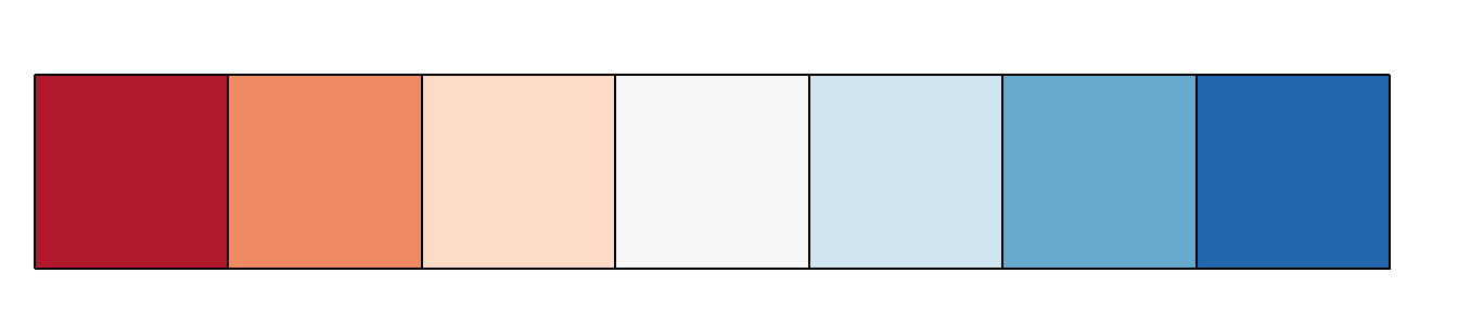
Quantitative schemes: use color gradient with two hues for positive and negative values. Gradient should go through a light, neutral color (white)
Small objects or thin lines need more contrast than larger areas
R package based on Cynthia Brewer’s color schemes